English
 Views: 0 Author: Elsa Long Publish Time: 2026-10-18 Origin: Site


Every panel that crosses a stencil printer carries a measurement report nobody reads. The printer logs its pressures, speeds, alignment solutions and cleaning cycles; the inspection machine behind it logs the volume, height and position of every deposit it measures. Together those logs describe the print process far more faithfully than any monthly defect meeting does — but only for the lines that have learned to work with them. The equipment itself is the easy part: the I.C.T solder paste printing machine lineup already outputs the data this guide discusses. The hard part is the discipline of turning logged numbers into control limits, and control limits into decisions.
This guide is deliberately concrete. It walks through the actual data fields a print cell produces — pressure, speed, separation, alignment offsets, deposit volume, transfer efficiency, per-pad statistics — with units and typical magnitudes, then defines the SPC criteria that work for print data: which charts, which rules, which capability thresholds, and which measurement-system caveats. It then catalogues the software functions that make the analysis sustainable rather than a spreadsheet hobby, and closes with improvement scenarios drawn from real print floors. The goal is a solder paste printing data analysis program your team can actually run, not a concept deck.
Table of Contents
Every process step on an SMT line generates data, but they are not equally valuable. Placement and reflow happen after the board is already populated with components worth many times the bare panel; printing happens first, on a bare board, and it is the step with the widest machine parameter surface — pressure, speed, separation, alignment, cleaning — interacting with the most consumables: paste, stencil, squeegee, support tooling. That combination makes printing the line's largest variance contributor and, simultaneously, its best-instrumented process: the two machines involved log thousands of numbers per panel. The raw material for statistical process control is already being produced and mostly discarded.
Disciplined solder paste printing data analysis is the practice of stopping that discard. Done well, it converts the print cell's logs into control charts that answer "is the process behaving normally right now", capability indices that answer "can this process hold the tolerance this product needs", and correlations that answer "which knob moves which measurement". Those three answers cover most of what print process engineering actually does — and they do it with data that already exists, on machines already installed. The sections that follow specify the fields, the statistics and the software functions; this section first establishes why the effort pays and what maturity looks like.
Print losses come in three shapes, and each hides differently. Sudden losses — a misload, a stencil smear, an empty paste cartridge — announce themselves immediately as gross defects and are usually caught within a board or two; they are dramatic but cheap. Chronic losses are the expensive ones: a transfer efficiency that sits at 78% instead of 92% on one aperture family, a volume mean that runs at the low edge of specification, an offset distribution twice as wide as the machine's capability. Chronic losses never trigger an alarm because each board passes; they cost a fraction of a percent of yield on every panel, every day, for years. The third shape is drift — slow degradation from wearing blades, loading underwipes and relaxing rails — which converts healthy chronic performance into marginal performance over weeks.
The defining property of all three loss shapes is that they are invisible from the front panel and from casual inspection. A board that measured 82% of target volume will reflow into an acceptable joint most of the time, so no operator call is made; the loss surfaces later as reflow defects scattered across products, days and operators in a pattern nobody can connect. Data analysis is what connects it: volume trended by stencil serial, transfer efficiency trended by aperture ratio, offset spread trended by rail service date. Each connection turns an invisible chronic loss into an addressed engineering item — which is why the analysis program's value concentrates on exactly the losses that are hardest to see any other way.
Print data programs mature in recognizable stages, and knowing the stages prevents two opposite failures: trying to run before crawling, and never getting past crawling. Level one is counting: the machine's own screens and counters — stroke counts, cleaning counts, alarm histories — read by humans and written into logs. Level one captures sudden failures and supports the maintenance checklist, but it sees nothing chronic. Level two is trending: inspection data and machine parameters exported and charted over time — volume means, offset spreads, Cpk by product. Level two is where chronic losses become visible and where most of this guide's value lives; it requires export capability and a review cadence but no special infrastructure. Level three is modeling: correlating parameters against measurements across products, building response models, and closing automatic correction loops.
The staging discipline matters because each level feeds the next. Level-three correlation models are only as good as the level-two trend history that supplies their training data, and level-two charts are only trustworthy if the level-one counters and records identify what changed and when. Lines that skip ahead — enabling automatic correction on a process that has no baseline — get oscillation, as the print-process guide's integration chapters warn. Lines that never leave level one pay for instrumentation they never use. The realistic ambition for most lines is a solid level two within a quarter and selective level three on the one or two products where the economics justify the modeling effort.
The returns are concrete and worth stating in operational terms. Defect triage compresses from hours to minutes: when a reflow defect appears, the SPI record of the deposit that produced it either convicts or exonerates the print step immediately, ending the three-department argument before it starts. Consumable life is managed on evidence: blade changes, stencil retirement and cleaning intervals tune to measured wear rates instead of calendar habit, which typically finds money on both sides — intervals that were too long and intervals that were needlessly short. New product introduction gets faster: the print response model built on one product family transfers to the next, so the first article prints closer to target and the tuning loop is shorter.
There is a procurement corollary worth noting: data capability is a machine feature, not an afterthought. Platforms differ in what they log, how it exports, and whether third-party SPC tools can read it — and once a line has built its analysis practice, that capability becomes part of the buying criteria for the next printer. Evaluating a solder paste printer for an SMT production line on data grounds means asking which parameters are logged at what resolution, whether inspection data can be correlated against them by serial or timestamp, and what the export path looks like — the same questions this guide's software section turns into a checklist.
Conceptual discussions of "print data" are useless for building an SPC program; the program is built on named fields with units, sampling rates and failure signatures. This section inventories those fields as they actually exist on modern equipment — first the machine-side process parameters that describe what was done, then the deposit-side inspection measurements that describe what resulted, and finally the context fields that make correlation possible. The tables are written to be lifted directly into a data dictionary: they are the schema of a solder paste printing data analysis program, and every field listed is produced by current-generation I.C.T printers and the SPI machines that pair with them.
One structural note before the tables: the machine-side and deposit-side streams must be joinable. A volume trend with no record of the pressure that produced it is half a dataset; the join key — timestamp, board serial, or panel ID — is the single most important "field" in the whole system, and its integrity is what the software section will spend most of its effort on. With the join in place, each table below becomes more than a list: each row is a control chart waiting to be drawn and a failure signature waiting to be matched.
Machine-side fields describe what the printer actually did, as distinct from what the recipe requested. The distinction matters because recipes state intent while logs state fact — and the gap between them is where many print problems live: pressure that sags under flow, speed that the drive never actually reaches, separation that differs between front and back of the stroke. A sound data dictionary therefore distinguishes setpoint fields (what the recipe says) from achieved fields (what the machine reports doing), and the SPC program charts the achieved values. The core inventory:
Field | Source | Units | Typical magnitude | Primary SPC use |
|---|---|---|---|---|
Squeegee pressure (achieved) | Pressure regulator / sensor | kg (or N) | 6–10 kg, guard-band ±0.5 | X-bar chart per shift; drift → blade wear or pneumatics |
Print speed | Recipe / drive feedback | mm/s | 20–80 mm/s | Changeover verification; correlation with fill |
Squeegee drop depth | Recipe / Z-axis | mm (0.01 res.) | −0.5 to −2.5 mm | Blade-contact gauge for new stencils |
Separation distance | Recipe | mm | 0.3–3.0 mm (or speed-based) | Recipe check; fine-pitch sensitivity |
Separation speed | Recipe | mm/s | 0.5–5 mm/s | Correlation with peak-volume defects |
Alignment offset X / Y / θ | Vision system | mm / deg | ±0.025 mm typical | I-MR chart; widening spread → rails, support |
Alignment time | Vision system | s | 3–10 s | Throughput budget; low-confidence FID warnings |
Underwipe interval & count | Cleaning system | prints | every 5–25 prints | Pairing with volume-variance trend |
Stencil / blade stroke count | Machine counters | strokes (cum.) | 10³–10⁵ range | Consumable-life evidence; wear-rate tracking |
Paste dwell time | MES / operator log | h | 0–8 h per batch | Correlation with end-of-batch volume decline |
Two fields in this table deserve special status. Achieved squeegee pressure is the machine-side field most predictive of deposit trouble and the one most often logged but never charted — give it a control chart in week one of any program. And alignment offset is the field most often misused: it is tempting to treat a shifting offset as a vision problem, but the offset mean and the offset spread diagnose different subsystems (a moving mean points at transport or support; a widening spread at rails or clamping), so chart both separately from day one.
The inspection stream is the dataset's payoff, and its fields are geometric and standardized across most 3D SPI platforms: volume, height and area per pad, plus positional offset, plus classifier flags for bridging and smearing. What turns these from inspection outputs into SPC inputs is aggregation discipline — per-pad values rolled up to per-board statistics, per-board statistics rolled to per-shift control charts, always keeping the traceability from any aggregate back down to the individual pads that composed it. The core inventory, with the acceptance conventions most paste suppliers publish:
Field | Units | Typical limits | What it diagnoses |
|---|---|---|---|
Deposit volume (% of aperture target) | % | 80–150% per paste spec | Overall process health; the headline chart |
Absolute volume per pad | µm³ (or nL) | product-specific | Per-pad baselines; small-aperture watch list |
Deposit height | µm | stencil ±30% | Slumping, scooping, gasket failure |
Printed area | % of pad | 80–120% | Spreading, bridging precursor, smear onset |
X / Y offset vs. pad | µm | ±25 µm typical | Transport, support and rail drift |
Transfer efficiency | % | 60–100% by aperture ratio | Fill quality on fine apertures; blade/stencil wear |
Bridging / smear flags | boolean | — | Pareto by product, stencil, zone |
Per-pad volume Cpk | — | ≥1.33 target | Product health score; release criterion |
Transfer efficiency earns a note because it is the field that makes consumable conversations quantitative. Volume percentage alone conflates aperture design with process performance; transfer efficiency — deposit volume as a fraction of the aperture's theoretical volume — normalizes for design, so a falling transfer efficiency on a specific aperture family is directly an argument about blade condition, paste rheology or foil quality, not about the product. The pairing of these measurement streams with the correction channels they can drive is worked through in detail in the printer–SPI closed-loop feedback reference; for SPC purposes, treat it as the deposit-side field with the cleanest cause-and-effect narrative.
The third field class carries no process values of its own but multiplies the value of everything else, because it is what makes correlation possible. Each printed panel should be attributable to: paste batch and mix time; stencil serial with its cumulative print count; blade ID and stroke count; underwipe roll or solvent age; board surface finish and batch; operator and shift; and ambient temperature and humidity. None of these fields is exotic — every modern printer and MES can carry them — but programs routinely omit two or three, and the omitted ones are always exactly the ones the first serious drift investigation needs.
The ambient pair is worth defending because it is the most commonly dropped. Paste rheology responds to temperature and humidity measurably within a single shift's range, and volume charts that ignore the ambient context regularly misattribute seasonal drift to consumables — a winter of "worn blades" that was actually dry air. Recording ambient at panel level costs nothing on machines with environment sensors and one manual reading per shift where they are absent. The test of a context schema is simple: when the next unexplained trend appears, can you answer "what else changed?" from the records alone? If the answer requires asking three people what they remember, the schema is incomplete.
Fields differ in how often they change and how long they stay useful, and the program should be explicit about both. Deposit measurements arrive at full rate — every pad of every board — and their aggregates are what get charted; retaining per-pad detail for thirty to ninety days is enough for drill-downs without unbounded storage. Machine-side achieved parameters change per stroke and should be logged per panel at minimum, per stroke where bandwidth allows. Context fields change per product, per batch or per shift, and belong on the same join key as the rest. Retention policy follows the investigation horizon: long enough to compare this month's Cpk against last quarter's baseline, short enough that the database stays queryable.
One rate trap deserves a warning: averaging is not sampling. A line that logs only per-shift averages of pressure has destroyed exactly the information SPC needs — the within-shift variation that distinguishes a machine drifting slowly from a machine oscillating between strokes. Where storage or interfaces force a choice, keep raw achieved values for a shorter window rather than averages for a longer one, because variation is the signal and the average is what remains after the signal is subtracted. This single decision separates programs whose charts detect problems in a shift from programs that discover problems at the quarterly review.
SPC is where solder paste printing data analysis either becomes an engineering discipline or degenerates into dashboards nobody trusts, and the difference lies in choosing statistics that match the data's actual structure. Print data is not one statistical animal: deposit volume behaves like a classic continuous measurement with subgroups, offset data is a pair of coordinates plus an angle, classifier flags are attributes, and several machine parameters are recipe-set values whose "variation" is mostly human. Applying one chart type to everything is the most common way good data gets wasted. This section defines the working statistical toolkit: which statistics per field, which chart per statistic, which detection rules, and what capability targets actually mean for print tolerances.
The section also carries a warning that belongs before the formulas: statistical machinery amplifies whatever it is fed, including measurement error. Before any control chart earns decision authority, the measurement system producing its numbers needs a verified repeatability figure — a gauge study on the SPI machine against known reference deposits, repeated on your paste and foil, not on the vendor's demo kit. An SPI machine with 8% gauge error will happily draw control limits around noise and set the process chasing phantom drift. The order is non-negotiable: verify the gauge, then baseline the process, then let the rules act.

The matching rule is simple: the statistic must preserve the information the decision needs. For deposit volume, the decision is "is the process centered and stable against the paste specification's window", which makes per-board mean and extreme the working pair — the mean watches centering, the extreme (worst-pad volume) watches the tail that actually produces defects. For alignment offset, the decision is "is the transport delivering boards consistently", which makes the offset mean and the offset standard deviation separate charts, because as noted earlier they diagnose different subsystems. For transfer efficiency, the decision is per-aperture-class, so the statistic is computed per aperture ratio band, not pooled — pooling hides exactly the small-aperture weakness the measurement exists to expose.
Attribute data — bridging flags, smear flags, fiducial failures — gets the attribute toolkit: p-charts or np-charts at board level, and, more usefully, a Pareto discipline by product, stencil and zone that turns the flag stream into a ranked work list. Machine-side achieved parameters get individuals charts (I-MR) because they arrive one value per panel with no natural subgroup. The worst statistical choices in print programs are all mismatches of this kind: charting per-pad volumes individually (thousands of correlated points that shred control limits), pooling aperture classes in transfer efficiency, or applying variables-chart rules to boolean flags. None of these are exotic errors; all of them are weekly occurrences in programs built by enthusiasm instead of by this section's table.
Quantity | Statistic | Chart | Detection rule | Standing response |
|---|---|---|---|---|
Deposit volume | Board mean + worst-pad % | X̄-R (subgroup = board) | ±3σ; 2-of-3 beyond 2σ; 8-point run | Bounded offset correction; escalate at rule break |
Transfer efficiency | Mean per aperture band | I-MR per band | ±3σ; 6-point trend | Blade/stencil review; paste rheology check |
Offset X / Y | Board mean; board σ | I-MR × 2 | ±3σ on both mean and σ | Mean moves → support/transport; spread widens → rails |
Squeegee pressure (achieved) | Per-panel value | I-MR | ±3σ; 9-point one side | Pneumatics / regulator check within shift |
Bridging / smear flags | Flag rate per shift | p-chart | Beyond limits; run rules | Pareto by stencil & zone; cleaning interval review |
Per-pad volume Cpk | Rolling 30-day | Trend line | <1.33 sustained 2 weeks | Product review; process redesign conversation |
Control limits come from the process, not from the specification — the single most violated principle in factory SPC. Limits are computed as the historical process mean plus and minus three sigma of the within-subgroup variation, using a baseline window of clean data (typically twenty to twenty-five boards per product after changeover). Limits drawn from specification windows produce charts that scream whenever the process sits off-center, and teams respond by muting alarms, which is how SPC programs die. Limits recomputed whenever the recipe, paste, stencil or blade materially changes — because those are new processes wearing old names — and the re-computation event itself is logged with its reason.
Detection rules should start minimal and grow only with proven need. The three worth having from day one: any point beyond a control limit; two of three consecutive points beyond the same two-sigma zone; and eight consecutive points on one side of the centerline. Western Electric-style supplemental rules (trends, strata, stratification patterns) earn their place only where the team has demonstrated the discipline to disposition each signal the same day it fires. An un-dispositioned signal is worse than a missed one — it trains the whole shift that the charts are decorative. The review cadence in Section 6 exists precisely to keep every signal attached to a disposition and a name.
Capability answers the question control charts cannot: granted the process is stable, can it hold this product's tolerance? For print data the working indices are Cp and Cpk on deposit volume against the paste specification's window, computed per product on a rolling window (thirty days is a common convention), with the short-term/long-term pair — Cpk and Ppk — reported together because their gap is itself diagnostic: a large gap means a stable process that drifts between setups, pointing at changeover discipline rather than machine physics. The customary acceptance bar is Cpk ≥ 1.33 for standard products and ≥ 1.67 where the product's reflow window is thin — 0201-class passives, 0.3 mm-pitch packages, large LED panels where rework economics are brutal.
Two print-specific cautions keep capability numbers honest. First, capability on volume must be computed per aperture class, not pooled across the board: a product whose fine apertures run Cpk 1.1 and whose large pads run 2.0 reports a pooled 1.6 that is fiction, and the fiction collapses at reflow. Second, the tolerance window matters as much as the measurement: capability against the paste vendor's generic window is a different claim than capability against the window your reflow profile actually tolerates, and the two should be reconciled once per paste change rather than assumed. Programs that report a single pooled Cpk for the plant are, statistically speaking, reporting nothing.
Gauge repeatability and reproducibility (GR&R) is the unglamorous prerequisite that separates working programs from confident nonsense, and on the print cell it has two parts. The SPI side: reference boards or known-geometry deposits measured repeatedly, across operators and days, to establish the gauge's sigma on your paste color, foil finish and pad geometry — the numbers that go into every sigma calculation downstream. The machine-parameter side is lighter but real: a pressure gauge's calibration status, a vision system's alignment repeatability test (Section 6 of the maintenance checklist covers the procedure), a speed readout verified once against a tachometer reference. A field with unknown gauge error cannot be charted with decision authority; it can be watched, but its signals route to verification, not to action.
The practical GR&R standard for SPI in print SPC is a total gauge sigma below 10% of the tolerance window — tighter for fine-pitch products where the window itself is narrow. When a gauge study fails, the remediation order is lighting and lens condition first (the maintenance checklist's optics tier), calibration second, and only then platform escalation, because most failing gauges in working factories are dirty or mis-calibrated rather than inadequate. Re-run the gauge study whenever paste color, board finish or stencil material changes materially — the measurement system's performance is conditional on exactly those variables, and a gauge verified on one product is not automatically verified on the next.
Data that never reaches an actuator, a work order or a design change is entertainment, so this section maps the measurements of Section 2 to the actions they can legitimately drive. The mapping matters because misrouted actions are how data programs lose credibility: sending a volume problem to the alignment actuator, or an offset problem to the pressure regulator, teaches the line that the charts are not worth reading. The catalog has three tiers with different authorities — automatic bounded corrections, human-triggered maintenance and consumable actions, and design-side feedback that changes the product or tooling rather than the process — and each tier has its own data prerequisites and its own failure modes.
The tier structure also disciplines expectations. Automatic correction is the most visible capability and the least broadly applicable: it works only where a parameter has a demonstrated, monotonic, fast response on the metric being corrected — which in practice means offset correction first, bounded volume corrections second, and a short list beyond that. Maintenance triggers are where most of the chronic-loss money is recovered, and they are available to every line regardless of automation level. Design-side feedback is the slowest tier and the largest payer: transfer-efficiency data routed to aperture design has probably returned more yield than every automatic correction combined, precisely because it fixes causes the process never could.
The automatic tier works on three proven channels. Offset correction — feeding measured X/Y/θ error back into the alignment reference — is mature, fast and safe within bounds, and should be the first channel enabled on any line. Volume corrections to pressure and print speed are the second channel, legitimate only after a designed experiment has established the response curve for the product family, and only with dead bands (a minimum signal before acting), persistence rules (a signal must repeat before the machine responds) and bounded step sizes. Separation-speed corrections for peak-profile defects are the third, narrower channel. Everything else — every tempting "the machine could fix this itself" extension — waits for the response model that justifies it, and the print-process guide's phase discipline (baseline, then limits, then corrections) is the roadmap for earning each channel.
The catalog's most important word is bounded. Every automatic correction carries a maximum step, a correction budget per shift, and an escalation condition under which the loop stops and hands the problem to a human, and those bounds are logged alongside the corrections they permitted. An unbounded loop is a machine confidently acting on its own worst measurement — the failure mode the entire discipline exists to prevent. Lines auditing their logs quarterly will find that bounded loops mostly correct in small amounts and escalate rarely, which is exactly the signature of a healthy one; a loop that uses its full correction budget daily is not correcting, it is compensating for a problem the data is trying to name.
The trigger tier converts the same measurements into work orders, and it is where print data pays most reliably. Volume variance trending up across two review cycles routes to the underwipe and stencil inspection; transfer efficiency declining on a specific aperture band routes to blade condition and paste rheology; offset spread widening routes to rail and clamping service; per-pad nonuniformity growing routes to the support-flatness check. Each trigger carries the evidence trail that makes the work order persuasive — the chart, the window, the magnitude — and each closes with a re-measurement confirming the fix, which is how the trigger list itself gets tuned over quarters. The solder paste printer preventive maintenance checklist defines the tiered cycles and the condition-based pairing mechanics in full; the SPC program's job here is to keep the signals honest and the dispositions logged.
Consumable life management is the trigger tier's quieter and equally valuable function. Stroke counters paired with measured blade wear, stencil print counts paired with tension and transfer-efficiency history, and solvent age paired with cleaning-effectiveness data turn consumable budgets from argument into arithmetic. The typical first-year finding is that one or two intervals were substantially wrong in each direction — a blade interval wasting usable life, an underwipe solvent interval silently degrading fine-pitch volumes — and each correction recurs as savings every cycle thereafter. This is also the data that ends the perennial consumable-brand argument: two stencils compared on the same line, same products, same charts, produce a verdict no meeting can overrule.
The third tier routes evidence outward to the people who design the stencil and the pad, and it is the tier with the highest ceiling. Transfer-efficiency data by aperture ratio, aggregated over months, is precisely the dataset a stencil designer needs to decide where foil thickness should change, where apertures need geometry modification, and where the process genuinely cannot fill the design as drawn. Offset and coplanarity data by board zone directs support-tooling design for the next fixture. Bridging Pareto data by pad geometry identifies the land-pattern details that generate chronic flags regardless of process settings. None of these problems were solvable by parameter tuning — that is why they persisted — and all of them become addressable once the data arrives in the designer's language.
Making the tier work is a routing discipline rather than a technical one. Each recurring data finding gets a disposition class — process, consumable, maintenance or design — and design-class findings accumulate into a quarterly package with the charts attached, sent to the stencil supplier or the CAD owner with the specific apertures and panels named. Suppliers respond to quantified arguments: "improve the small apertures" is a wish, while "aperture class B runs 71% mean transfer efficiency against 88% for class C on identical paste and blade conditions across six weeks" is a specification. The stencil and squeegee consumable selection guide for stencil foils and squeegee blades covers the design parameters themselves; the data program's contribution is making those conversations quantitative and periodic instead of anecdotal and occasional.
The analysis program lives or dies on its software path, because discipline that depends on hand-copying numbers dies within a month. This section defines what the software must actually do, in four layers: connectivity (getting the data out of the machines), the SPC engine (charting, rules, capability), the review layer (dashboards and views that make the weekly session efficient), and the evaluation checklist for judging any tool — including the software that ships on the machines themselves. The layer structure is deliberate: a line can assemble a working program from machine-native tools plus one export path and a spreadsheet, and many should start exactly there; the checklist tells you what you are missing and when the upgrade pays.
Modern printers differ sharply in native data capability, and the differences are a legitimate purchasing criterion. A fully automatic platform such as the I.C.T fully automatic SMT PCB stencil screen printer carries the complete field set from Section 2 — achieved parameters, counters, cleaning logs, alignment records — with network export designed in, while compact and semi-automatic platforms expose smaller but still SPC-usable subsets, often over USB export or a local network share. The program's first software decision is simply making an inventory: which of the Section 2 fields each installed machine actually exposes, at what resolution, over what interface. Everything downstream is sized against that inventory.

The connectivity layer has one hard requirement — a join key — and one soft requirement — a cadence that does not depend on anyone's memory. The join key (timestamp plus board serial, or panel ID) is what lets a deposit measurement be paired with the machine state that produced it; without it, the two streams are two half-datasets, and no amount of downstream software repairs the loss. Export cadence matters because manual exports happen when someone remembers: the working patterns are automatic file drops to a network share (most platforms support CSV or XML export per shift or per panel), direct database writes where the line's MES provides a schema, or machine-to-machine streams for closed-loop pairs. Whatever the path, its health is itself monitored — an export that silently stopped two weeks ago is the most common way data programs rot.
Protocol reality is worth stating plainly because vendor material obscures it. SMEMA, the line's universal transport handshake, carries board flow only — it is not a data protocol, and the presence of SMEMA says nothing about data capability. Machine-to-machine data channels ride the factory network over ordinary mechanisms — file shares, OPC UA, vendor APIs, or MES schemas like those IPC's connectivity standards describe — and what matters for evaluation is which of those the machine actually implements and what fields each carries, in writing, before purchase. For closed-loop printer–SPI pairs the data channel carries corrections as well as measurements, which raises the stakes on clock alignment and recipe synchronization; the integration guide's architecture section maps those requirements in detail.
The engine layer turns the joined dataset into the statistical outputs of Section 3, and its requirement list is short but strict: control charts with limits computed from process baselines (not specification windows), the detection rules of Section 3 implemented as configurable options, capability indices computed per product and per aperture class on rolling windows, and drill-down from any aggregate point to the underlying boards and pads. Two features separate serious engines from chart libraries: limit-change management (limits recomputed on recipe or material change events, with the event logged) and signal dispositioning (each rule-break carries a disposition, an owner and a closure state, queryable later). A chart without dispositioning is a photograph; the disposition log is what turns six months of charts into process knowledge.
Correlation tooling lives at this layer's upper edge and is the level-three capability from Section 1: scatter and regression of deposit metrics against machine parameters across products, with product and aperture-class filtering. It does not need to be sophisticated — a scatter of board-mean volume against achieved pressure, filterable by stencil serial, answers most of the questions correlation tooling ever actually gets asked — but it needs to exist inside the same tool as the charts, because the question always arises mid-review, and exporting to another tool kills the moment. Lines that outgrow this and move to response-surface modeling and automatic closed-loop correction are usually ready for the MES-grade analytics tier, which is a procurement conversation with different economics, not a software feature to bolt on gradually.
The review layer's design question is what the weekly session needs to see, and the answer is a small number of curated views, not a wall of charts. The working set: a product health page (current Cpk, volume mean trend, flag Pareto per product), a machine health page (achieved-parameter charts, alignment repeatability, cleaning-cycle logs per printer), and a signals page (open dispositions, aging, owners). Every view drill-downs to board and pad level, because the session's most common question is "show me the actual deposits behind that point". Dashboards that fail in practice share the same flaws: too many charts, no drill-down, and no linkage between a signal and its disposition state — visual enthusiasm wrapping an unactionable surface.
The operator-facing view is a different artifact and worth building separately: a single screen per printer showing current status against the shift's expectations — last-board statistics, cleaning cycles due, any open signal for that machine — with the deliberate omission of everything the operator cannot act on. High-volume platforms such as the I.C.T 1200 mm LED PCB fully automatic paste printing machine run panels whose scrap economics make minutes matter, and the operator view's job is to surface the one thing that needs attention now, not to reproduce the engineer's analytics on a shop-floor screen. The two views share a database and differ in everything else, including vocabulary.
Whether evaluating the machine's native software, a third-party SPC package, or the spreadsheet-plus-export stopgap, the same checklist applies, and it fits on one page. Data: which Section 2 fields are ingested, at what rate, with what join key, and what happens when a source is offline. Statistics: baselined limits, rule configuration, per-class capability, drill-down. Workflow: dispositioning with owners and closure, limit-change events logged, weekly-review export. Operations: retention policy, backup, query performance at real volumes, and who administers it. Cost honesty: the spreadsheet stopgap is genuinely viable at level two for a single line — its ceiling is multi-line aggregation and audit readiness, not daily analysis, and knowing when that ceiling is reached is part of the plan, not an accident.
For most programs the realistic path is staged: native machine software plus one reliable export and a disciplined spreadsheet in the first quarter; a dedicated SPC tool when the second line, the second product family, or the first audit arrives; MES-grade analytics only when multi-line correlation and closed-loop scale make the economics obvious. The software section of the maintenance and records framework pairs naturally with this checklist — the PM records and the SPC data share the same join keys and the same review cadence, and programs that unify them early avoid rebuilding both when the CMMS and the SPC tool need to talk.
Capability | Minimum viable | Full program | Why it matters |
|---|---|---|---|
Data path | Shift CSV export to share | Automated panel-level writes with join key | Discipline that depends on memory dies |
Charts & rules | I-MR / X̄-R, ±3σ, run rules | Configurable rules, limit-change events | Baselined limits, not spec windows |
Capability | Cpk per product, rolling 30-day | Per aperture class, Cpk/Ppk pair | Pooled Cpk reports nothing |
Drill-down | Point → board → pads | Full traceability incl. corrections | The review's most common question |
Dispositioning | Log with owner + closure | Queryable, aging alerts | Charts become knowledge, not photos |
Retention & admin | Named owner, backup | Retention policy, audit exports | Rot and loss are silent |
Software produces charts; only people produce improvement, and the operating model — who reviews what, on which rhythm, with what authority — is what keeps the program alive after the launch energy fades. The operating model has three roles and three rhythms, and it is deliberately lightweight: a program that needs a meeting to function has already grown too heavy for the print floor. The roles are the operator (who acts on the machine-facing view and escalates signals), the process owner (a named engineer who owns limits, dispositions and the weekly review), and the maintenance interface (the technician tier that receives routed work orders with their evidence attached).
The rhythms are a shift check, a weekly review, and a monthly capability report. Each rhythm has a defined artifact and a defined duration, and both are short: the shift check is minutes, the weekly review is thirty to forty-five minutes against the three dashboard views, and the monthly report is a one-page capability summary per product. Everything else — dashboards, correlation tools, trigger lists — exists to make those three rhythms fast. When a review starts generating hour-long debates about chart validity, that is the operating model telling you the measurement-system work of Section 3 has been skipped, and the fix is back in the gauge study, not in another meeting.
The operator's authority is narrow and precise: act on what the machine-facing view says (cleaning due, material at end of life, a signal the machine flags for acknowledgment), and escalate anything that needs judgment. The process owner holds the statistical authority: adjusting limits, dispositioning signals, authorizing corrections, and deciding when a product's charts have earned rule changes. The maintenance interface receives routed work orders and returns re-measurement evidence. The ladder matters because the two failure modes are mirror images: operators making statistical decisions they lack context for (muting alarms to keep the line running), and process owners hoarding decisions the operator could close in seconds. Written role definitions of one page each, reviewed at onboarding, prevent both.
Equipment class shapes the operator's role more than anything else in the operating model. On a semi-automatic platform such as the I.C.T semi-automatic vacuum screen solder paste printer, the operator is close to the process on every stroke and functions as a genuine sensor — their observations belong in the disposition log alongside the charts. On a fully automatic line the operator manages several machines at once and interacts through exception views only. Compact desktop cells such as the I.C.T desktop SMD stencil printer with pick-and-place and reflow often put one person across the whole line, in which case the operating model collapses gracefully: the same person holds operator and process-owner roles with the review rhythm compressed to a daily fifteen minutes. The model serves the line, not the other way around.
The weekly review is the program's heartbeat, and its shape is worth specifying exactly. Thirty to forty-five minutes, standing agenda: every open signal since last week, each with its chart, its disposition status and its owner — closed signals get their re-measurement confirmed, open ones get an aging check (anything past two weeks escalates automatically); then the product health page, product by product, with the Cpk trend and any limit-change events reviewed; then one correlation question, brought by whoever has one, worked in the tool rather than on a whiteboard. The output is a written disposition log entry per signal — which is the artifact that compounds into process knowledge over quarters.
Two disciplines keep the review from decaying. First, no signal leaves without a disposition class: process (a parameter to change), consumable (a life item to order), maintenance (a work order routed) or design (routed to the quarterly package from Section 4). Second, the review audits itself monthly: how many signals fired, how many were dispositioned on time, how many re-measurements confirmed their fixes. A review whose audit shows ninety percent on-time dispositions is a working program; one at fifty percent has become a meeting, and the remedies are structural — fewer rules, tighter triggers, or a co-owner sharing the load — not exhortation.
The monthly capability report is the program's external face, and it should fit on one page per product: current Cpk with its trend arrow, volume mean against the paste window, flag rates with their Pareto leaders, and the month's limit changes with reasons. This is the artifact that satisfies auditors, informs customers, and — less visibly — forces the process owner to look at each product's whole picture once a month, which the weekly view's signal-focus can miss. The report's data comes directly from the disposition log and the rolling capability windows; a report that requires manual assembly is a report that will be late, and lateness is how reporting rhythms die.
The audit trail is the quiet deliverable that distinguishes a program from a practice. Every limit change, every disposition, every correction the loop applied, every override a human made — timestamped, attributed, queryable. Modern platforms store most of this natively; the operating model's contribution is the discipline that completes it (the disposition log) and the retention policy that keeps it (the Section 2 field-lifecycle rules). When a customer quality engineer asks how print quality is assured, the answer is a fifteen-minute query, and that answer wins business more often than any brochure claim about the machines involved.
Framework sections convince nobody; scenarios do. This closing section walks three improvement arcs drawn from common print-floor situations, each traced through the pipeline this guide built — fields, statistics, software, action — with the actual numbers an engineer would see. The scenarios are composites of recurring patterns rather than case studies of specific customers, chosen because between them they cover the three loss shapes from Section 1: a chronic loss, a drift loss, and a product-introduction loss. Read them as worked examples: the same pipeline, run three times, on three different problems.
Each scenario also names the fields and charts that carried the diagnosis, so the examples double as a walkthrough of the earlier sections — if a step in the story is unclear, the section it cites supplies the machinery. And because the arcs are composites, the numbers are realistic rather than exceptional: the improvement magnitudes shown here are what the pipeline delivers on ordinary lines with ordinary problems, not the showcase results vendors lead with. That is the point. This discipline's returns come from closing ordinary losses permanently, not from heroics, and the compounding effect in the third scenario is the honest shape of the payback.
A line runs a mixed-product schedule on a semi-auto platform paired with a bench SPI machine for sampling. The first month of the program produces the baseline: board-mean volume sits at 96% of target — inside specification, no flags anywhere — but the per-aperture-class breakdown shows fine apertures (0.3 mm class) running a mean transfer efficiency of 74% against 91% for the 0.5 mm class, with a class Cpk of 1.12. Nothing about this was visible before, because nothing about it breaks: boards pass, AOI finds no pattern, and the print step has been quietly consuming margin on every fine-pitch panel for a year.
The correlation work is one afternoon: transfer efficiency by aperture class, filtered by stencil serial, overlaid with the blade stroke count. The fine-aperture efficiency declines with stroke count within each stencil's life and recovers at blade change — a blade-lip wear signature concentrated exactly where fill pressure margins are thinnest. The action catalog routes it to both human tiers: blade inspection interval tightens for this product family, and the quarterly design package carries the aperture-class transfer table to the stencil supplier, who proposes a step-down foil thickness for the fine-aperture region. Ninety days later the class runs 88% transfer efficiency at Cpk 1.51 — the chronic loss is closed on both the process and design sides, and the evidence trail is the whole story.
A mid-volume line running a dependable semi-automatic platform — the workhorse class represented by the I.C.T semi-auto stencil printer for SMT PCB paste printing — starts showing a slow widening of the offset spread on its flagship product: three weeks of drift, unremarkable per day, a spread 40% wider than baseline by month's end. The offset mean is steady, so the vision system is exonerated by the two-chart rule from Section 3; bridging flags rise in parallel, concentrated at board edge zones. The alarm instinct says paste, and the paste supplier has already been called.
The drift's direction — spread, not mean; edges, not center — routes the investigation to the transport and support tier before anyone opens a paste jar. The machine logs show underwipe solvent age in range, but the maintenance records show the width-repeatability check from the monthly PM suite skipped during a two-week maintenance staffing gap. The verification is run: width repeatability has doubled its baseline spread, and rail inspection finds debris packed at the guide corners. Rail service, verification print, and the offset spread returns to baseline within a shift — and the paste supplier call is quietly cancelled. The diagnostic discipline that saved the day is pure structure: mean and spread charted separately, context fields attached, escalation routed by failure signature rather than by instinct.
A contract manufacturer introduces a dense new board — fine-pitch on both sides of the panel — and the print tuning conversation starts from data rather than habit, because the previous product's program left a baseline. The response model built on the old product predicts the pressure and speed window for the new foil; the first article prints at 103% mean volume with a per-class Cpk of 1.21 — close, but short of the 1.33 gate the program requires for release. The gap concentrates in one aperture family again, and this time the tuning loop is short: separation speed adjusted within the predicted window, verified by the SPI pairing, gate met on the fourth trial build rather than the tenth.
The quieter win is the design package that goes back with the release: the new product's aperture-class transfer table, with one land-pattern flagged for the next board revision at Cpk 1.28 — acceptable, but flagged as the first thing to widen if the product's volume grows. That is the maturity arc of the whole discipline in miniature: the first program month bought a baseline, the baseline bought a model, the model bought a faster release, and the release's own data bought the next improvement before anyone felt pain. A solder paste printing data analysis program's return follows exactly this compounding shape — slow, then structural, then permanent.
Turn your print data into a working SPC program
Everything in this guide assumes machines that log honestly and export cleanly — and that is exactly where I.C.T engineers spend their time with customers: auditing which of the Section 2 fields your installed base actually exposes, mapping the export path, and building the baseline windows that make control limits real. If you are starting a solder paste printing data analysis program, recovering a stalled one, or specifying your next printer with data capability on the list, bring us your field inventory and your worst trend chart. We will return a staged plan — what to chart in week one, which triggers to route first, and where the software gaps genuinely need closing — matched to your products, your volumes and the inspection platform you already run.
The conversation starts with your data rather than our catalog: send one week of export in any format, even partial, plus the product that worries you most, and we will show you what the fields reveal, which of the action tiers from Section 4 apply immediately, and what the staged plan looks like for your line. The data is already flowing; the program is the discipline layer on top, and it starts with one chart next week.
Four, in this order: board-mean deposit volume (X̄-R chart), achieved squeegee pressure (I-MR), alignment offset mean and spread (two separate I-MR charts), and bridging flag rate per shift (p-chart). These four cover the highest-frequency failure signatures and require nothing beyond native machine logs plus SPI export. Add transfer efficiency per aperture class as the fifth once the join key is proven — it is the most diagnostic of the consumable conversations.
No. Sampled inspection supports level-two trending honestly as long as the charts say so — control limits from sampled data describe the sample, and rare events pass unseen. What sampling cannot support is automatic correction, which needs per-panel measurements. Many programs run sampled SPI for months, build their baselines and trigger discipline, and then justify inline inspection on the signal density the sampling showed them they were missing. Start with what you have; the statistics do not change.
The working convention is Cpk ≥ 1.33 against the paste specification's volume window for standard products, and ≥ 1.67 for thin-window applications — 0201-class parts, 0.3 mm pitch, or products whose reflow profile tolerates little volume error. Compute per aperture class, never pooled, and report the Cpk/Ppk pair so the setup-to-setup gap is visible. A capability number that fails the per-class test is a summary, not a capability claim.
On a join key: timestamp plus board serial is the standard pair, carried identically on both streams. Verify the clocks on both machines against the same source — a five-minute clock skew silently misjoins every correlation. Where the MES assigns panel IDs, use those; where it does not, the printer's per-panel sequence number plus date is a workable key. Test the join on one day of real data before building anything on top of it — mismatched keys are the most common reason correlation work "shows nothing".
For one line at level two, genuinely yes: CSV export, charted columns, manually maintained limit baselines and a disposition tab will run a disciplined program for months. The ceiling is aggregation across lines, audit-ready traceability, and rule automation — when the second line arrives, or dispositions start living in someone's inbox, migrate. The failure mode is not the spreadsheet; it is the spreadsheet outliving its validity because nobody defined the migration trigger.
Start with three: any point beyond a control limit, two of three consecutive points in the same two-sigma zone, and eight consecutive points on one side of the centerline. Every fired signal must receive a same-day disposition — a rule without the discipline to answer it teaches the line that charts are decorative. Add Western Electric supplemental rules only when the team has demonstrated it closes signals reliably, and retire rules that fire repeatedly without actionable findings.
Most SPI packages chart the inspection stream well but see only one side of the process: they lack the machine-side achieved parameters, the maintenance counters and the context fields that make cause-and-effect work possible. The analysis program's distinctive value is the join — deposit measurements paired with the machine state that produced them. If your SPI software can ingest machine-side data with a join key, extend it; if it cannot, export both streams and join them in the SPC layer rather than surrendering the correlation capability.
They share the same join keys, the same counter fields and the same review cadence, and they should be designed together: the SPC trend data is what turns calendar-based maintenance into condition-based triggers, while the maintenance records provide the "what changed" events that explain chart movements. Lines that run them separately rebuild the same data schema twice and lose the correlation between service events and process shifts — which is precisely the correlation that makes both programs smarter.