English
Views: 0 Author: Elsa Long Publish Time: 2026-10-21 Origin: Site


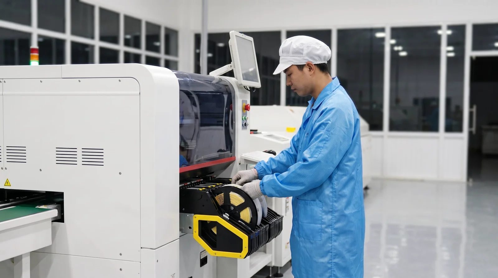
The placement machine is the heart of any assembly line, and the moment a project gets serious about one, the datasheets all start to look alike: gantries, spindles, a rated CPH number, an accuracy figure. What the datasheet cannot do is tell you which machine your project actually needs, because that answer lives in your own files — in the bill of materials, the board outline, the feeder count, the delivery schedule and the budget you have to defend. This guide builds that bridge. It takes the six inputs every real project carries — BOM, PCB size, component range, feeder needs, throughput and budget — and turns them into a step-by-step framework for selecting among the Hanwha DECAN S1, S2, F2 and L2, the models you can browse in the full I.C.T pick and place machine range.
How to choose a Hanwha pick and place machine is therefore not a question with a single answer, but a sequence of decisions that narrow the field logically: component requirements first, because they are the least negotiable; model capability second, because that is where the range separates; board handling and feeders next, because they decide how the machine fits the line; then throughput and budget, which confirm the choice can actually be defended. Each section of this guide takes one of those decisions in order, works through the trade-offs a process engineer would weigh, and closes with the checklists and calculations that turn a shortlist into a signed purchase order.
Table of Contents
Every placement machine purchase starts the same way: someone opens three or four datasheets side by side and compares the numbers that are easiest to compare — placement rate, accuracy, component range. The problem is that this comparison cannot produce a decision, because it never references the project. Two lines with identical rated throughput can have completely different real output if one builds boards with four thousand passives and the other builds boards with four hundred; two machines with identical accuracy ratings can produce different yields if one project runs 03015 components and the other never goes below 0402. The datasheet describes what a machine can do in principle; only the project describes what it must do in practice. That is why the discipline this guide follows is to derive every requirement from a project input before any model is named.
The framework has six inputs, and each one eliminates or confirms something specific. The BOM defines what the machine must be able to place at all. The PCB size defines what it must physically carry. The component range sets the accuracy class and the head technology. Feeder needs determine configuration and changeover behavior. Throughput converts those capabilities into a rate the schedule can be planned against, and budget closes the loop by forcing the trade-offs to be made explicitly rather than silently. The sub-sections below explain how to collect and read each input, so that by the time the DECAN models appear in section three, the choice among them is arithmetic rather than debate — which is exactly how to choose a Hanwha pick and place machine under real project pressure.
Before any model discussion, the selection team should fill in a one-page project profile containing six rows. The BOM row lists total placements per board, split by component class: chips, fine-pitch ICs, connectors, odd-form parts. The PCB row records board length and width, thickness range, and whether boards run singly or in panels. The component-range row names the smallest chip package, the finest lead pitch, and the largest or longest component the project must handle. The feeder row counts tape, tray and stick quantities per board and per product family. The throughput row states required boards per hour per shift, and the budget row states the capital envelope with its timeline. None of these rows is difficult to fill; what makes the exercise valuable is that together they answer every question the vendor will ask, in the order that matters.
The table below summarizes the six inputs and what each one decides. Used this way, the profile becomes the contract between the project team and the equipment supplier: any candidate that fails one row is out, and any candidate that passes all six is a legitimate option to price. The discipline also shortens supplier meetings, because the conversation moves from "what do you need?" — a question that produces vague answers — to "does this configuration meet these numbers?", a question that produces commitments.
Project input | What you record | What it decides |
|---|---|---|
BOM | Placements per board by component class | Placement volume, head and nozzle mix |
PCB size | Length, width, thickness, panel strategy | Board envelope, rail and support configuration |
Component range | Smallest chip, finest pitch, longest part | Accuracy class, vision capability, model tier |
Feeder needs | Tape, tray and stick counts per product | Feeder capacity, banks, changeover method |
Throughput | Required boards per hour per shift | Single machine vs dual module, line count |
Budget | Capital envelope and timeline | Configuration level, new vs phased purchase |
Datasheets are written to be comparable, and that very quality makes them misleading without context. A rated placement rate is measured under conditions optimized for the measurement: identical chips, minimal travel, no vision steps. A real product mixes packages, forces the head to fly between distant coordinates, and inserts vision correction and tray pickups that never appear in the rated number. The standardized way to compare machines is the IPC-9850 placement equipment performance verification, which defines how placement speed and accuracy are measured and reported; it makes datasheets honest, but it still measures a reference board, not yours. The gap between the verified figure and your line's output is not vendor deception — it is geometry and mix, and it is calculable if you know your BOM.
The practical rule is to treat every datasheet number as a capacity ceiling, never as a plan. Accuracy figures follow the same logic: a machine's stated placement precision applies across its supported component range, but the margin you need depends on what you place. The same ±30-micron class capability that is generous for 0603 chips becomes a working minimum for 03015 packages or 0.3 mm-pitch ICs, and only your component list can tell you which side of that line you are on. Reading a datasheet project-first therefore means annotating each specification with the BOM line that stresses it hardest — and rejecting any candidate that cannot answer that annotation with a specific, verifiable figure.
The most common selection error in this equipment class is buying the fastest machine in the budget and discovering the constraint was elsewhere. A high-speed placer bolted into a line whose printer or oven paces it will simply idle, and the extra capacity is paid for in capital and consumed in depreciation. The opposite error is just as real: a line built around flexible but slower machines that cannot absorb the volume growth the sales plan assumes, forcing an early second line purchase that a better-balanced first line would have delayed. Both errors come from treating placement rate as the single axis of the decision, when it is one of six inputs and rarely the binding one.
Speed-first selection also distorts the mix of capabilities a line actually needs. Boards with heavy connectors, tall modules or long LED components punish machines optimized purely for chip rate, and the yield loss on those components quietly eats the advantage the rated speed promised. The corrective is to cost the errors, not just the machine: estimate what one point of first-pass yield is worth per year on your volume, and what one hour of changeover downtime costs per changeover, then weigh any speed advantage against the capability differences that affect those two numbers. A framework that runs the six inputs in order makes this comparison routine, and it is the reason the framework — not the headline CPH — is the asset this guide wants to leave you with.
The remaining sections follow the six inputs in decision order. Section two starts from the BOM and component range, because those define the machine class no budget argument can override: a project that must place 03015 chips or fine-pitch ICs is shopping in a different tier than one placing 0603s and SOICs, regardless of throughput. Section three maps those requirements onto the DECAN S1, S2, F2 and L2, giving each model a profile — which projects it fits, which it overshoots, and where its configuration flexibility matters. Section four covers PCB size, paneling and board handling; section five covers feeders, setup and changeover, the domain where high-mix lines win or lose their schedules.
Sections six and seven close the financial loop. Section six converts rated CPH into a realistic placement rate for your boards, with a worked calculation you can copy into a spreadsheet, and shows how to balance the line around the placer rather than discovering the balance after commissioning. Section seven handles budget: what the purchase price includes and excludes, how total cost of ownership behaves over five years, and how to match a budget tier to production reality without starving capability. The guide closes with a decision checklist and answers to the questions buyers most often ask. Read once in order, it is a tutorial; thereafter, the tables and checklists are designed to be used standalone on each new project.
The bill of materials is the ground truth of every placement decision, and it should be read twice: once for volume and once for difficulty. The volume read is arithmetic — sum the placements per board across the products the line will run, and the result sizes the throughput requirement in section six. The difficulty read is more consequential: it identifies the components that constrain machine choice, the ones a lesser machine either cannot place or cannot place reliably. Those constraint components — the smallest chips, the finest pitches, the longest connectors, the heaviest modules — matter far more than the average, because a machine that places 99% of a board well and fails on the remaining 1% produces boards that cannot ship. Component range is therefore the first filter, and it is applied before any model is considered.
This section organizes the BOM read into three analyses. It examines the fine-pitch and micro-chip end of the range, where placement accuracy and vision capability are tested hardest. It then covers the long-component and odd-form end, where feeders, grippers and machine envelope matter more than speed. Finally, it shows how to compress the whole BOM into a component-range matrix — a short table that any supplier can be held to — so the requirement travels with the project rather than living in one engineer's experience.
At the difficult end of the passive range, package size stops being a specification detail and becomes the tier marker. The DECAN platform places components from 03015 upward — among the smallest chip packages in volume electronics — and crossing that threshold changes the meaning of every other number on the datasheet. At 03015 scale, placement accuracy tolerances of roughly ±25 to ±30 microns are not a comfort margin but the operating band, nozzle design becomes specialized, and feeder presentation precision matters as much as head precision, because a chip mis-presented at the pick is already a defect before it reaches the board. A project containing such packages should treat them as the anchor requirement the rest of the selection is built around.
Fine-pitch ICs impose a parallel requirement through their leads. Packages at 0.4 mm pitch and below need not only positional accuracy but vision systems that can find and correct for lead variation, plus stable flight-path control so the part arrives level. This is also where the acceptability criteria of IPC-A-610 become a production constraint rather than an inspection formality: offset, solder-joint geometry and tombstoning risk all scale with placement precision, and rework on fine-pitch devices costs multiples of the placement. The disciplined question for every candidate machine is therefore not "what is the accuracy?" but "what is the accuracy, verified, on the smallest and finest components in my BOM, at my board's complexity?" — and the answer should come with a demonstration, not a datasheet page.
The other end of the BOM eliminates machines just as decisively. Battery holders, shields, keyed connectors, electrolytic capacitors above a certain diameter, transformers and module assemblies exceed what a standard tape feeder presents, and each class stresses a different capability: length tests the placement head's Z-stroke and vision field, weight tests holding force and release control, and irregular shapes test whether the machine supports special nozzles or gripper tooling. Hanwha's DECAN L2 is the model in the range built for exactly this class of work — its multi-functional head and support for large connectors up to approximately 75 mm in length make it the default answer for BOMs where odd-form content is structural rather than occasional, and the DECAN L2 multi-functional placer product page details that capability in the machine's own numbers.
Odd-form capability also changes how the rest of the line should be planned, and this is where BOM analysis connects to line design. A board dominated by power devices is a different project from a dense consumer board even at identical placement counts, because component mass, thermal design and inspection all shift. Teams planning such products should read the BOM alongside our guide to choosing an SMT line for power electronics PCBA, which walks the same project-first method for the whole line. The selection rule this section leaves you with is simple: count the components no ordinary machine places well, assign each a target machine capability, and let those few BOM lines — not the thousands of routine chips — choose the model tier.
The output of the BOM read should be one table short enough to fax to a supplier and specific enough to hold them to. List every component class the project runs, and against each class record four things: the extreme case in your current BOMs (smallest package, finest pitch, longest body, greatest mass), the quantity per board, the feeder type it arrives on, and the process risk if placement is marginal. Compressing hundreds of line items into eight or ten classes takes an hour with a script and forces the team to agree on what "difficult" means for this project. That agreement is worth more than any datasheet, because it converts taste into requirements.
The matrix below is a starting template with the classes most BOMs contain. A consumer board and an industrial controller fill it very differently — the consumer board stresses the chip and fine-pitch rows, the industrial board stresses the connector and module rows — and that difference is precisely the information model selection needs. Once the matrix exists, every candidate machine is scored row by row: pass, conditional or fail, with the condition written down. Only machines that pass or conditionally pass every row advance to the throughput and budget stages, which keeps the later arithmetic honest.
Component class | Record the extreme case | Machine requirement it drives |
|---|---|---|
Micro chips | Smallest package, e.g. 03015 / 0201 | Accuracy class, specialized nozzles, precise feeders |
Standard chips | 0402–0603 volume share | Rated placement rate, feeder count |
Fine-pitch ICs | Finest lead pitch, e.g. 0.3–0.4 mm | Vision correction quality, flight-path control |
Large ICs / BGAs | Max body size and mass | Wide-component support, Z-stroke, holding force |
Connectors / long parts | Longest body, e.g. up to ~75 mm | Multi-functional head or gripper, special feeders |
Odd-form / modules | Heaviest or shaped part | Tray handling, tooling options, placement force control |
With the requirement side defined, the model landscape can be mapped onto it honestly. The Hanwha DECAN family spans four placements in the current I.C.T range, and each earns its place by solving a different project shape: the S2 is the flagship for raw placement rate, the F2 is the high-speed workhorse tuned for value, the L2 is the multi-functional specialist for long, heavy and LED-heavy boards, and the S1 is the single-gantry entry that brings the platform into smaller budgets. Rated placement rates across the range run from roughly 47,000 CPH on the S1 to about 92,000 CPH on the S2, with component capability from 03015 chips up to large connectors and modules — a spread wide enough that most projects have exactly one natural fit, provided the six inputs are known. The figure below shows the machine these numbers describe in its natural habitat: a production line, feeders loaded, run by the people who will live with the selection.

The comparison table below condenses the range into the six columns that matter for selection, using the vendors' rated figures — treat them as ceilings, as section one argued, and let the sub-sections translate each model into project language. One caution applies to every row: configuration options change what a model can do, so the table describes the platform position, not a substitute for a configuration review against your component-range matrix from section two.
Model | Gantries × spindles | Rated placement rate | Character | Natural project fit |
|---|---|---|---|---|
DECAN S2 | 2 × 10 | ~92,000 CPH | Flagship speed, full-range components | High-volume consumer and automotive boards, tight takt |
DECAN F2 | 2 × 10 | ~80,000 CPH | High-speed value class | Volume boards where rate matters and capital is bounded |
DECAN L2 | 2 × 6 | ~56,000 CPH | Multi-functional, long and LED-optimized | LED modules, long boards, connector-heavy industrial BOMs |
DECAN S1 | 1 × 10 | ~47,000 CPH | Single-gantry flexible entry | Mid-volume lines, first machine, high-mix growth paths |
The S2 and F2 share the platform's dual-gantry, ten-spindle-per-gantry architecture, and both exist to convert feeder capacity into boards per hour. The S2 sits at the top of the range with a rated placement rate of about 92,000 CPH, achieved by flying two gantries in coordinated opposition so that pick and place cycles overlap; it keeps the platform's full component range, from 03015 chips to roughly 40-millimeter square bodies, so speed does not cost capability at the difficult end of the BOM. That combination — top-tier rate without sacrificing micro-chip or fine-pitch capability — is why the S2 is the default answer for consumer-volume and automotive projects where takt time is set by the market rather than by the scheduler, and the Hanwha DECAN S2 high-speed placer page carries the machine's full configuration options.
The F2 occupies the adjacent position one tier down: the same dual-gantry, dual-ten-spindle layout and the same component philosophy, with a rated rate around 80,000 CPH. In practice the F2's role is to ask whether a project needs the last ten percent of headline speed or would rather deploy the budget difference elsewhere — feeders, a second machine, upstream automation. For many volume projects the honest answer is the latter, because section six will show that rated-rate differences shrink once real board mix is applied. Choosing between S2 and F2 is therefore not a hierarchy judgment but a takt calculation: derive the required placement rate from the schedule, apply the realistic-rate factor, and let the result — not the flagships' prestige — pick the machine.
The L2 trades spindle count for range. With dual gantries of six spindles each and a rated rate around 56,000 CPH, it is not the machine for dense consumer boards — and it is not trying to be. Its head and feeders are configured for the components other machines struggle with: long bodies up to approximately 75 millimeters, heavy modules, and the long PCB formats that lighting products demand, with lens-optimized vision support for LED placement work. For a lighting manufacturer, that combination usually makes the L2 the anchor of the line rather than one machine among many, and projects of that kind should read it together with our guide to an SMT production line for LED lighting manufacturing, which follows the same project-first logic line-wide.
The L2 also earns its place on industrial boards whose BOMs are connector-rich even when they are not LED-related, and here its value is quantifiable: every long or odd-form component a dedicated machine places in-line is a component that does not detour through manual placement or an off-line inserter, with all the yield and traceability benefits that implies. The selection test is the component-range matrix from section two — if the connector and module rows dominate, the L2 moves up the shortlist regardless of its mid-range placement rate, and if those rows are empty, it drops off just as fast. Model choice, again, is the BOM speaking.
The S1 carries the DECAN platform's capability into a single-gantry chassis, with a rated placement rate around 47,000 CPH. What it gives up in headline speed it keeps in capability: the same component philosophy from micro chips upward, the same accuracy class where it matters, and the same feeder ecosystem, which means a line that starts on an S1 can migrate up the range without reinvesting in feeders, software or operator knowledge. That migration path is the S1's real product. It fits the mid-volume project, the new line that must prove its schedule before expanding, and the high-mix shop whose boards are component-rich but placement-light — where capability per placement matters more than placements per hour, and the DECAN S1 single-gantry machine page shows the configuration range it shares with its stablemates.
The honest limitation is takt. A project whose realistic placement requirement exceeds what one gantry delivers per hour will outgrow the S1, and the correct reading of that risk is not to avoid the machine but to size the growth path explicitly: two S1 lines, or an upgrade to the dual-gantry tier, with the feeder stock and line layout planned so either future is cheap. Buyers who make that plan in writing at purchase time get the S1's budget advantage without its ceiling; buyers who ignore it buy the same machine twice. Section seven returns to this trade in budget terms, because it is the clearest example of capability, throughput and cost trading against each other in one decision.
Placement capability means nothing if the board cannot travel through the machine, and board handling is the requirement teams discover latest and regret hardest. It is discovered late because it looks trivial — a board is flat and rectangular, and rails are rails — and regretted hard because the failures are physical: a rail that will not close to the panel width, a support pin that cannot clear the bottom-side components, a conveyor that exceeds the line's length budget by centimeters. Board handling therefore deserves the same requirement discipline as component range: measure, record, and hold candidates to the record. Four sub-questions organize the work — envelope, paneling, support, and line integration — and each converts a physical property of the product into a machine specification.
The good news is that within one platform family, board handling is a configuration question rather than a model question: the DECAN models share rail concepts, support strategies and interface standards, differing in degrees rather than kinds. That makes this section's output a specification sheet the whole range is judged against, and it makes the few differences — in board size limits between models, for example — worth flagging explicitly in the supplier conversation rather than assuming parity.
Start with the honest dimensions: the largest board the line will run, measured including any panel framing, plus the tolerance the fabricator actually holds. Record length, width and thickness extremes across all products, present and roadmap, because an envelope sized to today's flagship product fails on next year's. Rails adjust to board width, but every adjustment mechanism has a range and a changeover cost — the time per width step, and whether the change is stored as a program recipe or performed by hand. A high-mix line changes widths constantly, and motorized, recipe-stored rail adjustment repays its cost in changeover minutes; a single-product line can live with simpler arrangements. The selection question is not "what is the maximum board size?" but "what is the maximum board size at my changeover frequency?"
Thickness and stiffness belong in the same record. Very thin boards and flex assemblies do not behave like rigid FR-4 on a conveyor: they need edge fixtures or carrier pallets, and the carrier strategy changes effective width, weight and loading height. Heavy copper-clad power boards add a different constraint — mass per board affects conveyor loading and stop-position accuracy, which in turn affects the placement coordinate the machine trusts. None of these is exotic, but all of them are cheaper to specify than to retrofit, and all of them belong on the same one-page record as the BOM matrix, so the supplier answers to a document rather than to a conversation.
Paneling is where board handling and throughput meet, and the decision deserves to be made at selection time rather than inherited from the fabricator. A 2×1 panel doubles the placements the machine processes per board stop, which cuts per-board edge time and rail-handling overhead — but it also doubles board size, which can cross an envelope limit, and it changes the support requirement under the panel's span. Depaneling at the end of line adds a process step with its own stress on the solder joints. The optimum is project-specific: high-placement-count small boards almost always justify paneling, while large boards with few placements often run cheaper singly, and the only way to know which side a product falls on is to run the takt arithmetic both ways.
The placement machine's role in the paneling decision is specific and often overlooked: fiducial strategy across the panel, the machine's ability to correct per-circuit within a panel, and bad-board marking all determine whether paneling gains the throughput it promises. A machine that must treat every circuit in a panel identically loses yield to one bad circuit; one that skips marked circuits converts the defect into throughput instead. These are software and vision capabilities, so they belong in the demonstration script, not just the datasheet read — bring a panel with a deliberately marked-out circuit and watch what the machine does with it.
Under the board, support is the quiet variable in placement accuracy. The placer places against a board whose position it trusts to the coordinate system established at fiducial recognition; if the board flexes under placement force, the trust is misplaced and the defect shows at fine-pitch components first. Support systems — programmable pin matrices, vacuum platens, dedicated magtrays — hold the span rigid, and their quality matters more as boards get thinner, larger or heavier at the edges. The requirement to record is the bottom-side topography: component heights and keep-out zones under the board, from which the support layout follows. A machine whose pin field cannot avoid the bottom-side connectors will place a warped board, and the resulting offsets will be diagnosed — expensively — as a machine accuracy problem that is really a support problem.
Flex and very thin substrates extend the same requirement into fixture territory. Carrier pallets standardize handling, protect the substrate and make width adjustment irrelevant, at the cost of pallet inventory and a cleaning logistics chain of their own. The selection question is whether the machine's rail and support geometry accepts the carrier at the required throughput, and whether carrier presence is detected and corrected for in the coordinate system. These are demonstrable behaviors: bring the thinnest, largest and heaviest sample boards to the demonstration, and score every candidate on what happens to all three — not on the demo board the supplier chose.
Finally, board handling extends beyond the machine frame to the line it joins. Conveyor heights must match the neighbors exactly, rails must align, and the handshaking that moves boards between machines runs on the SMEMA interface convention the industry standardized decades ago — simple, robust, and universal enough that integration risk concentrates in physical fit rather than protocol. Record line length available, conveyor height, and the direction of travel, then check each candidate's footprint against the record including doors, maintenance access and feeder-cart clearance, which datasheet footprints habitually omit. A machine that fits the pitch but blocks the feeder cart creates a permanent operational tax paid once per shift.
Integration also has an upstream and downstream dimension: how the placer signals the printer about board arrival and completion, whether the line controller can schedule around the placer's changeovers, and what traceability data the machine exports to the plant system. None of these decides the model choice by itself, but together they decide the cost of the first month of operation, and lines that skip the review pay for it in integration surprises during commissioning. The checklist in section seven includes these items precisely so they are asked at selection, when the supplier can still answer for free.
If the BOM decides what a machine can place, feeder capacity decides what it can place without stopping. Every component arrives at the placement machine on a feeder — tape reels, tray stacks, stick tubes — and the machine can only run a board whose complete feeder set is installed. That innocent sentence is the source of most high-mix scheduling pain: a board needing 120 feeder positions on a machine holding 96 cannot run at all, and a board needing 100 positions on a 120-position machine forces a choice between partial loading with mid-run intervention and full loading with idle positions. Feeder planning is therefore not an accessory decision; it is co-equal with model selection, and on high-mix lines it is the difference between a schedule that holds and one that slips board by board.
This section treats feeders in three passes. It counts the real feeder requirement from the BOM matrix, distinguishing per-board needs from per-product-family needs. It then examines how the machine's feeder banks, carts and software handle setup and changeover, where the same feeder count delivers very different productive hours depending on how quickly it can be reconfigured. Finally, it covers the nozzle and head side of the same problem, because feeder capacity and placement-head reach are two halves of one constraint. The figure below shows the environment these decisions shape.

The count starts from the BOM but must not end there. Per board, sum the distinct 8-millimeter tape feeders, then the wider tape widths, then the tray-fed components, and remember that two boards sharing a feeder set can load simultaneously, while two products alternating on the same machine cannot. The number that governs machine configuration is the maximum concurrent feeder demand across the product families that must change over fastest — a figure that is usually 30 to 50 percent above any single board's count. Undercounting here converts directly into mid-run feeder swaps, and a mid-run swap on a line producing boards per minute costs more in interrupted flow than the additional feeder positions cost in capital, which is why experienced buyers size the feeder bank to the family peak, not the board average.
Feeder type mix deserves equal attention. Tape covers the chip and IC majority on most boards, but tray-fed components — large ICs, connectors, modules — consume placement-head travel to a tray station and back, which affects takt in ways the feeder count alone hides. Stick-fed parts persist in some industrial and legacy BOMs and need their own presentation hardware. The disciplined output is a feeder census table: feeder type and width, quantity per family, and the peak concurrent total — the same one-page discipline as the component-range matrix, and the document the supplier's configuration engineer should be asked to satisfy in writing rather than in a meeting.
Two machines with identical feeder counts can differ enormously in how they spend a changeover, and the difference lives in the mechanics of setup. Fixed feeder banks are loaded in place: the machine stops, feeders are swapped by hand at the machine, and the line's productive hour pays for every minute. Off-line setup changes the economics — feeders are staged on carts or banks away from the line, verified and kitted for the next product, and the changeover becomes a swap of prepared assemblies rather than a feeding frenzy at the rail. The DECAN platform's cart-based setup support is designed for exactly this workflow, and its value scales with changeover frequency: a line changing products twice a shift is a different economic case from one changing twice a week, and only the first case justifies premium setup hardware on arithmetic alone.
Setup time is also a software number, not only a mechanical one. Recipe management that recalls feeder maps, nozzle assignments and program offsets as a unit; verification that scans the loaded bank and confirms each position against the recipe; and missing-feeder tolerance that lets a board run with known-empty positions are all standard expectations now, but their completeness varies by configuration and should be demonstrated, not assumed. The demonstration script should include a full changeover performed by the supplier's own people at production pace, timed from last good board to first good board — one number, more honest than any brochure sentence about "fast changeover," and directly comparable across every candidate on the shortlist.
The feeder question has a mirror on the head side: every component class a board demands, the head must be equipped to pick and place, and switching nozzles consumes cycles. The head's spindle count determines how many components travel per flight — ten spindles per gantry on the DECAN dual-gantry machines — but the effective number depends on nozzle mix, because a flight carrying nozzle changes or collecting from a distant tray delivers less than a flight cycling between tape and board. A BOM whose component classes span micro chips to long connectors needs a nozzle range to match, and automatic nozzle changers keep that range resident without manual intervention, preserving unattended running through mixed boards.
Nozzle economics continue after the purchase: nozzles are consumables with a life measured in placement cycles, they need scheduled cleaning and inspection to hold placement accuracy, and their spares stock is part of the real budget section seven accounts for. The selection-stage questions are capability questions: which nozzle range the configuration supports, how the changer sequences across the board's component classes, and what the vendor's own process data says about nozzle life on similar mixes. A supplier who answers those from maintenance records rather than brochures is telling you how the machine will behave in year two — which is the year the feeder and nozzle decisions either fade into routine or become the line's standing bottleneck.
Throughput is the input everyone writes down and the number most often misread, because the bridge between a rated placement rate and boards per hour on your product crosses territory the rating never measures. The rated figure is a ceiling measured under repetition-favorable conditions; your product adds travel distance, vision correction, tray pickups, panel handling and changeovers, and each deduction is calculable before purchase. Treating throughput as a calculation rather than a datasheet quote is what separates a line plan from a line hope, and this section provides the calculation in a form you can run on any candidate machine.
Three analyses make the number real. The first decomposes the gap between rated and realistic rates, showing where the minutes actually go. The second works the arithmetic on an example board, producing a planning figure you can defend in a capacity review. The third zooms out to the line, because a placer's output only matters at the rate the whole line absorbs it — and the balancing decisions that follow belong in the selection conversation, not after commissioning.
The rated placement rate assumes the geometry of a test board: components arranged to minimize head travel, a single package type to eliminate nozzle changes, and no measurement steps between pick and place. Real boards violate every assumption. Head travel stretches as components scatter across the board; vision correction adds per-component time exactly where accuracy matters most; tray pickups cost a flight each; and panel handling inserts rail time the rated number never sees. The IPC-9850 standard exists precisely because raw CPH claims are not comparable — it defines how placement performance is measured and reported, which makes vendor figures honest without making them predictive. Prediction is your job, and it is tractable, because the deductions have structure.
That structure is the efficiency factor: the ratio of real output to rated rate, and it behaves consistently by board type. Dense boards dominated by chips and small ICs run efficiently because flights fill and travel stays short — factors around 0.5 to 0.7 of rated are typical planning figures. Mixed boards with connectors, trays and vision-heavy ICs fall further, often 0.3 to 0.5. Odd-form-heavy industrial boards can fall below those bands when long components force single-component flights. The exact factor for your product comes from the calculation below, but the planning discipline starts here: never build a capacity plan on a rated rate, always on a rate derived from the board's own geometry, and demand that any supplier proposal show the same derivation on your data.
The calculation has four steps and takes half an hour with a real BOM. Step one: count placements per board by class — chips, ICs, connectors, tray parts. Step two: estimate flight composition, the number of placements per head flight for each class, which depends on nozzle mix and board layout; chip-dense regions deliver near the spindle count, scattered components deliver less. Step three: convert to cycle time by dividing placements by flights, then adding per-flight travel allowances — longer for scattered layouts, plus fixed allowances for tray visits and panel handling per board. Step four: divide the result into the available production seconds per shift, then subtract changeover time at the changeover frequency the schedule implies. The result is the boards-per-shift figure the plan should be built on.
The table below walks the arithmetic on an example board — a mixed industrial controller with 600 placements — on two machines from the range to show how the method separates candidates. The figures are illustrative planning numbers, not vendor ratings; the point is the method, which converts both machines' rated rates into the same currency: boards per shift on your product. A supplier can and should run this table with your BOM for every machine they propose, and the conversation that follows the table is where the real selection information lives.
Step | Example: 600-place industrial board | Planning note |
|---|---|---|
Rated rate (machine) | ~80,000 CPH class, e.g. DECAN F2 | Ceiling, not plan — see IPC-9850 caveat |
Efficiency factor | 0.4 (mixed board: chips + ICs + trays) | Dense boards 0.5–0.7, mixed 0.3–0.5 |
Realistic placement rate | 80,000 × 0.4 = 32,000 CPH | Product-specific planning figure |
Cycle time per board | 600 / 32,000 × 3,600 s ≈ 68 s | Add panel handling per board stop |
Boards per 7.5 h shift | ~370 before changeovers | Deduct changeovers at planned frequency |
Cross-check | Same BOM on ~92,000 CPH class (S2) | Higher factor headroom for growth, higher capital |
A placement plan is only as good as the line around it. If the realistic calculation says the F2-class machine delivers the required boards per shift with margin, the balancing question becomes whether the printer and reflow can absorb the same rate — and if the calculation says only the S2 class meets the schedule, the balance question applies with more urgency, because faster placers are cheaper than second lines. Balance also has a changeover dimension: a placer that can change over via off-line carts while the rest of the line holds buffers behaves, for scheduling purposes, like a faster machine, and that equivalence belongs in the capacity model. The DECAN F2 automatic pick and place machine and the flagship DECAN S2 are best compared at this level — as line components in a takt model — rather than as isolated datasheet rows.
Balancing ends with a decision rule worth writing down before purchase: define the margin the schedule must hold — commonly 20 to 30 percent above current demand — and require the selected configuration to clear it. Margin absorbs the mix drift every real product family drifts through, the efficiency decay between maintenance cycles, and the growth the sales plan promises. A line bought without margin runs at its ceiling from day one, and ceilings have a way of converting every process hiccup into a missed shipment. The projects that regret their placement purchase almost never regret buying too much margin; they regret discovering its absence after the first demand surge.
Budget is the input teams most often treat as a constraint and least often treat as an instrument. A capital envelope does not just cap the purchase; it forces every trade-off in the framework to be made explicitly — capability against rate, margin against configuration, feeder stock against headroom — and a project that hides those trade-offs inside an undocumented number will pay for them in change orders. The purpose of this section is to make the money conversation as structured as the technical one: what the purchase price includes and, more importantly, excludes; how the cost of ownership behaves over the first five years; and how to match a budget tier to production reality without starving the capability the BOM matrix demands. Handled this way, budget becomes the final filter on a shortlist already narrowed by engineering — the last step of how to choose a Hanwha pick and place machine, not the first.
The sub-sections build that structure in order. Price composition comes first, because the quote-to-invoice gap is where budgets die. Total cost of ownership follows, converting the purchase into a five-year figure that supports honest comparison across configurations and vendors. The third sub-section matches budget tiers to the production reality each tier actually fits, using the DECAN range as the worked example. The last assembles everything this guide has produced into a final checklist — the document to carry into the supplier meeting and the standard against which the eventual proposal should be scored.
A machine price quotes the cabinet, the head configuration and the base software; a working placement capability costs more, and the difference is predictable if you know what to ask for. The recurring exclusions are feeder hardware — often quoted per position, so a 120-position requirement can move the total by a meaningful fraction — nozzle sets for the full component range, setup carts, board-support tooling, and the spare-parts kit that keeps the first year of maintenance from turning into emergency freight. Software items matter equally: recipe management, off-line programming, and the traceability interface the plant system expects. Training and commissioning complete the list, and they are the exclusions with the highest regret coefficient, because a capable machine run by an unprepared team delivers a fraction of its rated value.
The disciplined response is a quote checklist, issued to every vendor, requiring line-item pricing for each of these categories on the same configuration basis. The comparison that follows is no longer between two tantalizing totals but between two complete cost pictures, and the completeness itself is diagnostic: a vendor who resists itemizing commissioning or spares is telling you where their margin hides. The checklist below in section 7.4 consolidates these items so nothing is asked twice, and the practice costs one email per vendor — the highest-return email in the purchase.
Five years is the honest horizon for placement equipment: long enough for consumables, maintenance and efficiency decay to matter, short enough that volume assumptions stay plausible. The TCO model adds to the purchase price five streams of cost. Energy and compressed air run continuously and vary more with configuration than with brand. Consumables — nozzles, filters, feeder wear parts — scale with placement volume, which makes them predictable from the throughput model in section six. Preventive maintenance follows the vendor's interval schedule and should be quoted per year, not discovered per incident. Downtime cost is the stream teams omit and regret: every unplanned stop costs the line its takt for the stop's duration, and the vendor's service response structure — local inventory, remote diagnostics, response-time commitments — prices that risk. Spares stock is the final stream, and it converts directly from the exclusions list above.
Set against these streams are the residual and the efficiency variables: a machine from a range with an active upgrade path retains value and accepts feeder stock forward, which the S1-to-dual-gantry migration described earlier makes concrete. Efficiency in the TCO model means real placement efficiency — the factor from section six — and it dwarfs most other line items: a configuration that runs at a 0.45 factor instead of 0.4 delivers the same output as a nominally faster machine, often at lower capital and lower consumable cost. That is the quiet argument for buying capability that fits the BOM over buying headline rate, and the TCO table is where that argument becomes arithmetic.
Budget tiers should be assigned by project shape, not by ambition. The entry tier — a single-gantry configuration such as the DECAN S1 — fits mid-volume lines, first machines proving a schedule, and high-mix shops whose capability needs outrun their placement counts; its budget advantage is real, and its growth path is contractual if you negotiate the feeder and software upgrade route at purchase. The volume tiers — the F2 and S2 — fit schedules whose takt the market sets, and the choice between them is the section-six calculation: buy the flagship only when the realistic-rate arithmetic, with margin, says the schedule needs it. The specialist tier — the L2 — fits LED and connector-heavy products, where it is frequently cheaper than any alternative that actually works.
The match becomes honest when the tier is tested against the margin rule from section six: 20 to 30 percent of headroom above current demand, held in the configuration as purchased. A tier that clears the rule is correctly sized; a tier that only meets today's demand is a deferred second purchase, and a tier far above the rule is capital parked idle. Both errors are common, and both are visible in one spreadsheet row if the model is built. The table below summarizes the tiers against the project shapes they fit — the final cross-reference between the framework's inputs and the range's answers.
Budget tier | Configuration class | Production reality it fits | Growth path |
|---|---|---|---|
Entry / mid-volume | Single gantry, ~47,000 CPH class (S1) | First line, high-mix, capability-led BOMs | Feeder and software carry forward to dual-gantry tier |
Volume value | Dual gantry, ~80,000 CPH class (F2) | Scheduled volume with bounded capital | Add second module or line |
Volume flagship | Dual gantry, ~92,000 CPH class (S2) | Market-set takt, tight margin on schedule | Line replication |
Specialist | Multi-functional, ~56,000 CPH class (L2) | LED, long boards, connector-heavy industrial | Paired with high-speed module for mixed plants |
Everything in this guide compresses to a one-page scorecard, and the scorecard is what the supplier meeting should fill in. It has six blocks mirroring the framework: BOM capability scored against the component-range matrix; board handling scored against the envelope record; feeder configuration scored against the census; throughput scored with the realistic-rate calculation on your BOM, at your changeover frequency; budget scored on the itemized quote and five-year TCO; and integration scored on the demonstration — including a changeover at production pace and the marked-bad-circuit panel test. Each block is pass, conditional or fail, with conditions written down and owned by the vendor in the proposal.
Two closing disciplines protect the scorecard's integrity. First, weigh quality outcomes explicitly: the placement accuracy and process capability that determine first-pass yield are audited downstream against IPC-A-610 workmanship criteria, so a machine that is marginal on your finest components is a yield decision, not a specification footnote. Second, time-box the decision: a shortlist that survives all six blocks is already rare, and extending the comparison for marginal gains costs schedule the capacity model says you do not have. When one candidate passes every block with conditions you find acceptable, the selection is made — and the framework that produced it is ready for the next project, which is the return on the discipline this guide has asked of you.
Checklist block | Evidence to require | Pass condition |
|---|---|---|
BOM capability | Demo on your finest-pitch and longest components | Matrix rows all pass or conditionally pass |
Board handling | Run of largest, thinnest, heaviest sample boards | Stable transport and support on all three |
Feeder configuration | Quote covering census peak, carts, verification | Family peak fits without mid-run swaps |
Throughput | Realistic-rate calculation on your BOM | Schedule + 20–30% margin cleared |
Budget & TCO | Itemized quote + five-year TCO model | No unpriced exclusions remain |
Integration | Timed changeover demo, panel skip test, SMEMA fit | All demonstrated, not asserted |
Match a Hanwha DECAN configuration to your project with I.C.T
The framework in this guide turns placement machine selection from a datasheet debate into a project calculation, and running that calculation on a real BOM is a conversation our engineers hold every week. Share your component-range matrix, board envelope record and feeder census, and we will run the realistic-rate model of section six against the DECAN S1, F2, S2 and L2 on your product — returning a configuration proposal with the throughput margin, feeder plan and itemized budget this guide's checklist requires. Whether the answer is the single-gantry flexibility of the S1, the volume value of the F2, the flagship rate of the S2 or the multi-functional reach of the L2, the recommendation arrives as evidence rather than assertion, exactly how to choose a Hanwha pick and place machine should end. Explore the full range on the I.C.T pick and place machine catalog, or send us your BOM summary and board outline to start the configuration review with a live demonstration on your own components — on site or by video — before any commitment is requested.
High-mix, low-volume shops usually fit the single-gantry tier: the DECAN S1 carries the platform's full component capability and feeder ecosystem at the range's entry point, and its feeder stock migrates forward if volume grows. The decision test is capability per placement, not placements per hour — a shop running connector-rich industrial boards with moderate placement counts needs the accuracy and range more than the rate, and how to choose a Hanwha pick and place machine in this context means sizing the feeder bank to the family peak and investing the budget difference in setup efficiency rather than headline speed.
Yes, within the DECAN platform's component envelope, but the configuration differs by emphasis. Micro chips demand the platform's highest accuracy class, specialized nozzles and precise feeder presentation; long connectors up to roughly 75 millimeters demand the multi-functional head and feeders the DECAN L2 is built around. A board containing both extremes should be demonstrated, not assumed: bring the smallest chip and the longest connector to the demonstration and require the machine to place both on the same program run, with the vision and nozzle-change sequence visible.
Count per board from the BOM, then size to the maximum concurrent demand across the product families that must change over fastest — typically 30 to 50 percent above any single board's count. A line that changes products several times per shift should also price off-line setup carts, because prepared, pre-verified feeder assemblies recover more productive hours than extra positions alone. The census table from section five is the document the supplier's configuration engineer should satisfy in writing.
Not directly, and no vendor intends it to be. Rated rates are measured on repetition-favorable test boards under the standardized IPC-9850 measurement discipline; real boards lose output to head travel, vision correction, tray pickups, panel handling and changeovers. Planning factors run roughly 0.5 to 0.7 of rated for chip-dense boards and 0.3 to 0.5 for mixed boards. Run the four-step calculation in section six on your own BOM, and require any proposal to show the same derivation — the comparison that follows is where honest machine selection happens.
LED products are the DECAN L2's designed territory: lens-optimized vision for LED placement, support for long PCB formats, and a multi-functional head that also covers the connectors and drivers LED assemblies carry. For lighting manufacturers, the placement decision usually anchors the whole line, so the board-handling and line-design questions around it are covered in our guide to SMT production lines for LED lighting manufacturing, and the L2 configuration should be demonstrated with your actual strip length and LED package.
Requirements are set by the package, not by preference. Packages at 0.4 millimeter pitch and below, and micro chips such as 03015, need the machine's top accuracy class — figures on the order of ±25 to ±30 microns — plus vision systems that correct for lead and body variation. The verification that matters is on your components: ask for measured placement performance on your finest-pitch package, then confirm the resulting offsets and solder joints meet the IPC-A-610 workmanship criteria your customer audits against. Accuracy that is marginal on paper becomes rework in production.
The answer comes from the margin rule and the changeover profile. One dual-gantry machine wins when takt is the constraint and changeovers are infrequent; two single-gantry machines win when products change over constantly, because one line can stage its next setup while the other runs, and when growth should be staged rather than committed. Model the schedule both ways with the section-six calculation — including changeover time at realistic frequency — and let the margin rule pick the configuration that clears it with the lower five-year cost.
Placement determines yield at its margins: micro chips misplaced tombstone or shade their neighbors, fine-pitch ICs placed with insufficient correction produce marginal joints that rework costs multiples to fix, and unsupported flex under placement force shifts coordinates the machine believes are true. A machine matched to the component-range matrix holds first-pass yield by construction; a machine marginal on the difficult rows converts every BOM difficulty into inspection escapes. That is why the framework weighs capability evidence — demonstrations on your components — above every other selection input.